A high standard-curve R² does not guarantee accurate concentrations

After measuring a set of standards, the software reports R²＝0.9996 and the curve looks straight. Yet results for low-concentration samples can still deviate substantially.

The issue is that R² describes the overall fit of the data; it cannot, by itself, demonstrate accurate measurement at every concentration. To decide whether a calibration curve is suitable for quantitation, examine deviations at individual levels, independent quality controls, and whether samples fall within a validated range.

This article discusses assays that use a calibration curve to calculate concentration, such as colorimetric protein assays and some fluorescence assays. The model, concentration range and acceptance criteria should follow the method and the intended use.

1 R² can approach 1 while a low-concentration point still deviates substantially

For ordinary least-squares regression with an intercept, R² measures how much of the overall variation in response is explained by the model. Across a broad concentration range, a deviation at the low end may be difficult to notice on the full-range plot.

Consider a set of teaching data:

The standard concentrations are 0, 1, 2, 5 and 10 μg/mL, with responses of 0, 0.12, 0.20, 0.50 and 1.00, respectively. These responses are used solely to demonstrate the calculation and are not assigned to a particular analytical method.

An unweighted simple linear fit with an intercept gives:

Response＝0.09920245×concentration＋0.00687117

R² is approximately 0.9996.

For the 1 μg/mL standard, substituting its response of 0.12 into the equation gives a back-calculated concentration of approximately 1.140 μg/mL, about 14.0% above the nominal concentration.

These are constructed teaching data, not measured product results. They demonstrate that an excellent overall fit can coexist with a substantial deviation at an individual low-concentration point. Whether 14.0% is acceptable depends on the method's predefined criteria.

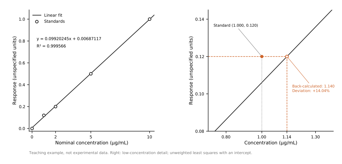
Figure 1 | Calibration curve and low-concentration detail. The teaching data are x=[0,1,2,5,10] μg/mL and y=[0,0.12,0.20,0.50,1.00]. Unweighted ordinary least-squares regression with an intercept gives R²=0.999566. The back-calculated concentration of the 1 μg/mL standard is 1.14038 μg/mL, a relative deviation of +14.04%. In the right panel, the filled orange point is the standard; the open point is the intersection of response 0.12 with the fitted line. These are not experimental data. Acceptance should follow the method's predefined criteria.

2 After the curve, examine residuals and back-calculation deviations

A residual is the measured response at a standard point minus the response predicted by the model. Plotting residuals against concentration often makes problems easier to identify than inspecting the fitted line alone.

Look for the following patterns:

• Residuals that follow a curved pattern with concentration: the current model may not adequately describe the response relationship.
• Greater residual spread at higher concentrations: measurement variability may differ across concentration levels.
• An individual point that deviates markedly: check preparation, sample addition, reaction and reading records.
• Residuals that change with measurement order: investigate possible drift in reaction timing or measurement conditions.

These patterns are diagnostic clues, not definitive causes. A lack of obvious structure in the residuals does not establish accuracy either.

Back-calculation more closely resembles using the calibration curve: treat each standard response as an unknown, calculate its concentration from the curve, and compare the result with its nominal value.

For nonzero standards:

Back-calculated relative deviation＝(back-calculated concentration－nominal concentration)÷nominal concentration×100%.

This formula cannot be used to calculate a relative deviation at zero concentration. Instead, examine the response, its variability and the method's blank requirements. Do not reduce deviations at different concentrations to a single average, which can conceal offsetting positive and negative deviations.

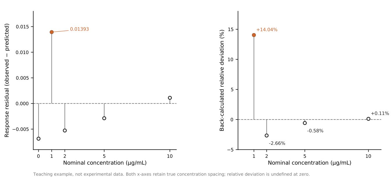
Figure 2 | Response residuals and back-calculated relative deviations for the same teaching data. Both horizontal axes preserve the actual concentration spacing. The back-calculated deviations for the nonzero standards are +14.04%, −2.66%, −0.58% and +0.11%, respectively; no relative deviation is calculated for the zero-concentration point. These are not experimental data.

3 After standards pass back-calculation checks, examine independent samples

The standards themselves contributed to the fit, so back-calculation mainly checks how well the model describes that data set. To assess reliability for other samples, use check samples that did not contribute to the fit.

One practical approach is to include quality-control samples at low, middle and high concentrations, process them in the same way as test samples, and assess their results against predefined criteria.

Where possible, quality-control samples should use independently prepared solutions. To investigate the assigned concentration or preparation of the calibration stock, also consider separately prepared stock solutions or other appropriate reference materials.

For example, suppose every standard has an actual concentration 10% above its label. The standards may still form a very straight line. Check samples prepared from the same stock may also fail to reveal this shared error.

Also distinguish two types of replication:

• Repeated readings of the same prepared solution mainly assess repeatability at the readout stage.
• Independent replicates starting from preparation, dilution or reaction are needed to include variability from those steps.

Stating where replication began is more informative than simply reporting “three replicates.”

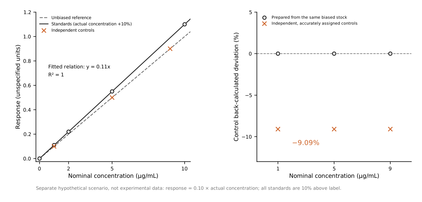
Figure 3 | Why a shared stock-solution error may escape detection by a high R² or same-stock controls. This is a separate idealized scenario, not the data in Figures 1 and 2: assume response=0.10×actual concentration and that every standard's actual concentration is 10% above its label. Fitting against the labels then gives y=0.11x and R²=1. Check samples prepared from the same biased stock have a back-calculated relative deviation of 0 from their nominal concentrations. Independent, accurately assigned controls at 1, 5 and 9 μg/mL back-calculate to 1/1.1 of their nominal concentrations, with relative deviations of −9.09%. The schematic ignores random error to explain the value of independent control sources; it does not represent actual method performance.

4 Do not alter the curve arbitrarily to increase R²

When a deviation is found, inspect experimental and data-processing records before deciding whether to adjust the model.

Do not force the fit through zero just to make the curve look straighter. Even after blank subtraction, check whether the remaining intercept is consistent with the method. Fixing the intercept requires experimental justification, not merely a tidy plot.

Do not treat deletion of standards as routine optimization. If a traceable preparation or handling error occurred, document the reason and follow predefined rules. Deleting a point solely because it lowers R² may make results look better without making them more trustworthy.

Do not select a more complex model on R² alone. A higher polynomial order may fit the existing points better while making predictions between them less stable. Model selection should also consider the response mechanism, residuals and independent checks.

Weighted fitting also requires justification. When measurement variability differs across concentrations, a weighted method may be assessed; weights should be supported by error characteristics and validation results, not chosen by trying alternatives until results “pass.”

5 What else is required when a sample falls within the calibration range?

A test sample's response falling between the lowest and highest standard responses is an important check, but it is not sufficient.

First, the interval should provide accuracy and precision suitable for the intended use. Detecting the lowest standard does not establish that its concentration can already be quantified reliably.

Second, standards and samples should be processed under comparable conditions. Differences in reaction time, temperature, sample-to-reagent ratio or sample matrix can affect response. Good performance in standard solutions does not automatically rule out interference in real samples.

Outside the validated range, do not simply extrapolate along the curve and report a reliable concentration. Adjust dilution or use another suitable range as permitted by the method, then measure again. Further dilution will generally not solve a result below the reliable quantitation limit.

Results from diluted samples must be converted back to the original concentration. Confirm whether the software has already applied the dilution factor to avoid multiplying twice. The dilution procedure itself should also be appropriately validated.

6 Answer at least six questions before using a curve

1. Are standard identity, concentration, units and dilution records clear?

2. Are the model, intercept treatment and weights justified?

3. Do residuals and back-calculation deviations at each concentration meet predefined requirements?

4. Do check samples not used in fitting give acceptable results?

5. Is the test sample within the validated range, without unevaluated matrix differences?

6. Are raw data, exception handling and the final calculation process fully retained?

Different experiments tolerate different levels of error. A single R² threshold should not be imposed on every method. Acceptance criteria should be established before the experiment and matched to the intended use.

A reliable calibration curve should make deviations, repeatability and check results across its applicable range visible. R² can remain in the report, but evidence for whether a concentration is usable needs to be more complete than one fit statistic.